Complete Guide To Descriptive Statistics in Python for Beginners

In the modern era, everything is now a data and data-driven system. Every second amount of data being generated is in terabytes. To draw meaningful statements and conclusions with numerical evidence, a widely used mathematics framework called Statistics is used.

So what is meant by statistics?

It means collection, organization, analysis and interpretation of data. Statistics are mainly used to give numerical conclusions. For example, if anyone asks you how many people are watching youtube, in this case, we can’t say more; many people are watching youtube, we have to answer in numerical terms that give more meaning to you. We can say like during weekdays 6 pm-8 pm more people are watching youtube applications and during weekend 8 pm-11 pm. If you want to answer active users, we can say there are two billion+ monthly active users, in the same way; the users spend a daily average of 18 minutes. This is the numerical way to conclude the questions, and statistics is the medium used to make such inference.

Statistics include;

Design of experiments: Used to understand Characteristics of the dataset
Sampling: Used to understand the samples
Descriptive statistics: Summarization of data
Inferential Statistics: Hypothesis way of concluding data
Probability Theory: Likelihood estimation

Why do we have to learn Statistics?

We are learning statistics because we can; observe the information properly, draw the conclusion from the large volume of the dataset, make reliable forecasts about business activity and improve the business process. To do all kinds of these analyses, statistics are used. Further, it is classified into two types: Descriptive and Inferential statistics.

Descriptive statistics summarize the data by computing mean, median, mode, standard deviation likewise. It is distinguished from inferential statistics by its aim to summarize the sample rather than use the data to learn more about the Population that; the sample of data thought to represent this means it is not developed based on probability theory.

Whereas inferential statistics are the methods for using sample data to make general conclusions (inferences) about populations by using the hypothesis. The sample is typically part of the whole population which contains only limited information about the population. For example, you might have seen the exit poll; those exit polls are calculated by taking several samples from different regions of that territory. Such conclusions are drawn from inferential statistics.

Descriptive statistics:

In statistical analysis, there are three main fundamental concepts associated with describing the data: location or Central tendency, Dissemination or spread, and Shape or distribution. A raw dataset is difficult to describe; descriptive statistics describe the dataset in a way simpler manner through;

The measure of central tendency (Mean, Median, Mode)

Measure of spread (Range, Quartile, Percentiles, absolute deviation, variance and standard deviation)

Measure of symmetry (Skewness)

Measure of Peakedness (Kurtosis)

Let’s see the above one by one by leveraging Python;

Code Implementation: Basic Statistics In Python

import pandas as pd
import matplotlib.pyplot as plt
dataset = pd.read_excel('3. Descriptive Statistics.xlsx',sheet_name=0)

Measures of central tendency:

The goal of central tendency is to come with the single value that best describes the distribution scores. There are three basic measurements used i.e, mean(the average value) , median(the middle value), mode(the most frequent value).

Let’s calculate the central tendency for the above example

Mean:

The arithmetic average of some data is the average score or value and is computed by simply adding all scores and dividing by the number of scores.

It uses information from every single score.

Here we are using python library pandas functionality to calculate most of our statistical parameters, so we don’t need to write code from scratch; it is just a matter of a few lines of code;

dataset[['CurrentSalary', 'After6Months', 'SalBegin']].mean()

The above says from 475 employees the average salary at beginning, After the six months and current as above. There are multiple types of means, such as weighted mean, trimmed mean but this is the most common use of mean.

Median:

Whenever we need to find a middle value, we go for the Median to calculate the median; we need to arrange values in ascending order. The median also attempts to define a typical value from the dataset, but unlike the mean, it does not require calculation, but it is a precaution while calculating the median like as;

If there are odd numbers of observations present in your dataset, then the median is the simple middle value of the ascending order of a particular column.

If there are even numbers of observations present, then the median value is the average of two middle values.

As we are using the Pandas library for the calculation, these precautionary things are handled automatically; as the methodology is concerned, we should know all these things.

dataset[['CurrentSalary', 'After6Months', 'SalBegin']].median()

The above values suggest at least half of the observations should have the current salary less than the 28875, in the same way, we conclude for the other two.

Mode:

The mode is used as the value that appears more frequently in our dataset. The institution of mode is not as immediate as mean or median, but there is a clear rationale. The mode value is usually being calculated for categorical variables. We can calculate mode by simply using .mode() to the pandas data frame object. The below is another way of calculating mode.

from collections import Counter
job_time = dataset['Job Time'].values
data = dict(Counter(job_time))
mode = [k for k, v in data.items() if v == max(list(data.values()))]
mode

The above code gives mode values like 93 and 81; this is a bit confusing right! This is because we have a tie between 93 and 81. After all, they are occurring in the same number.

These are all concepts in Measure of Central tendency.

The measure of dispersion (spread):

In this, we have different concepts such as Range, Standard Deviation, Variance, Quartile. However, it mainly tells how data is spread from the center, nothing but mean median, mode.

The range is nothing but the largest value subtracted from the lowest value. It ignores the effect of outliers, considers only two points in its estimation and does not recognize data distribution.

Next is deviation; the deviation is calculated to know how values have deviated from the mean. We can calculate the deviation for any central measures, i.e. mean, median, mode. While calculating deviation, we have to ignore negative values and consider them as positive.

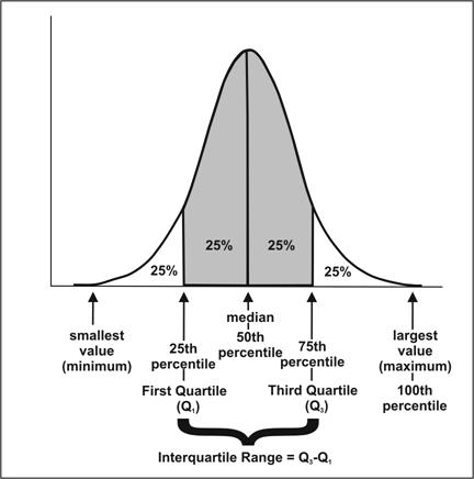
Quartile means quarterly basis calculations. Quartiles of distribution are the three values that split the data into four equal parts like as below where Q1 is 25th percentile, Q2 is 50th percentile, and Q3 is the 75th percentile;

The Interquartile range(IQR) is a measure that indicates the extent to which the central 50% values within the dataset are dispersed. It is calculated as Q3-Q1. As far as dealing with outliers is concerned, IQR can be used to impute the outliers values.

Next is variance, used mainly to find variation in the dataset. Variance indicates how close to or far from the mean are most of the values from a particular variable, and the standard deviation of the square root of the variance gives the magnitude of the variance. In other words, the standard deviation is used to check the consistency of the data lower the high-value consistency is there.

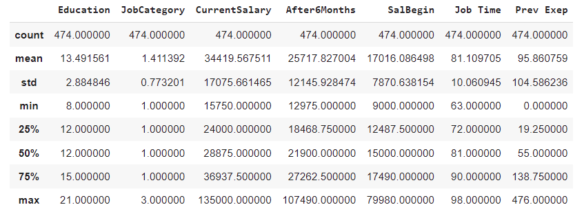
To calculate all the parameters under a measure of dispersion, we can code individually for all the parameters or use the NumPy package to do so. Here, as we are dealing with the data frame, the pandas .describe() function gives all of the parameters we need.

dataset[['Education', 'JobCategory',
       'CurrentSalary', 'After6Months', 'SalBegin', 'Job Time', 'Prev Exep']].describe(include='all')

The measure of symmetry and peakedness:

Skewness is the measure of symmetry or, more precisely, the lack of symmetry. For example, a distribution or dataset is symmetric if it looks the same to the left and right of the data of the centre point.

Whereas kurtosis is the measure of whether the data are heavy-tailed or light-tailed relative to normal distribution. This means datasets with high kurtosis tend to have more data points on either side.

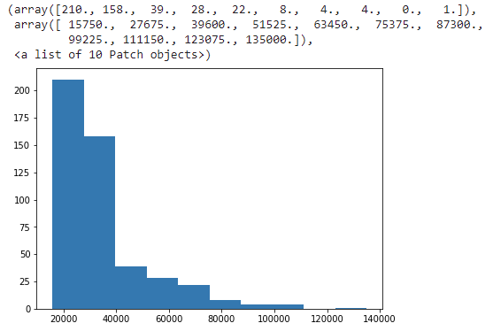
The histogram is an effective graphical way to show both skewness and kurtosis;

plt.figure(figsize=(7,5))
plt.hist(dataset.CurrentSalary)

The data is +vely skewed from the above histogram, i.e. mean > median; it has a heavy tail which means data contains more outliers.

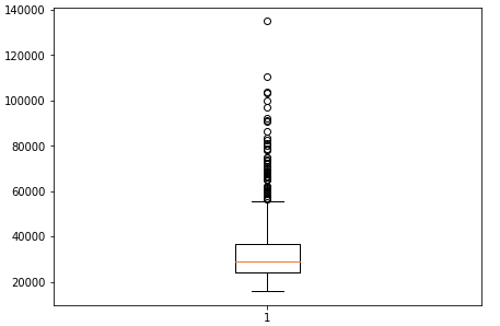
To see the distribution of the outliers, we can scatter plot or box plot, which gives a clear representation of data. Boxplot can be treated as an option to the histogram as it gives nearly all the information as histogram gives.

plt.figure(figsize=(7,5))
plt.boxplot(dataset.CurrentSalary)

Conclusion:

This was all about the basics of statistics, especially descriptive statistics. The above concepts of descriptive statistics help in: identifying potential data problems such as error outliers, identifying the process issues, selecting appropriate statistical tests for understanding the underlying relationship or pattern. Here we have used the pandas package to calculate all the parameters. We can also use packages like NumPy, math modules or can code it from scratch.

References:

The post Complete Guide To Descriptive Statistics in Python for Beginners appeared first on Analytics India Magazine.