The objective of this article is to evaluate different techniques for time series forecasting. These techniques include OLS model, Co-integration model and ARIMAX model
Business problem: To forecast the different components of PPNR. These components include Non-interest Income and Non-interest Expense.
Proposed solution
OLSModel
Co-IntModel
ARIMAXModel
Notes
Preference
High
Medium
Low
Complexity
Low
Medium
High
Dependent variable is stationary
OLS should be used
ARIMAX should be used
For ARIMAX both (dependent and independent variables) should be stationary together
Independent variable is stationary
Dependent variable is non-stationary
Co-Int should be used
ARIMAX should be used
For ARIMAX both (dependent and independent variables) should be non-stationary together
Independent variable is non-stationary
Auto-correlation
DW test close to 2
DW test close to 2
DW test close to 2
If for OLS or Co-integration DW fails then ARIMAX should be used
Variable significance
p-value < 0.05
p-value < 0.05
p-value < 0.05
For ARIMAX the AR, MA and exogenous terms should be significant
Multi co-linearity
VIF < 5
VIF < 5
VIF < 5
Residual is stationary
ADF test should pass
ADF test should pass
ADF test should pass
Residual is non-stationary
For all the three approaches, the residual should be stationary
Normality and homoscedasticity of residual
Should pass
Should pass
Should pass
OLS
Advantages – easy to develop / test and easy to explain
Disadvantages– difficult to finding strong correlation between dependent and independent variables
Co-Integration
Advantages – easy to find strong correlations between dependent and independent variables
Disadvantages – difficult to pass all the tests / assumptions of co-integration
ARIMAX
Advantages – very powerful modeling technique to overcome the shortcomings of OLS and co-integration models
Disadvantages – complex to develop as there are two stages. In stage 1 OLS model is developed and in stage 2 ARIMAX model is developed post identification of AR and MA terms
Introduction
PPNR
Pre-provision net revenue (PPNR), under the Federal Reserve’s Comprehensive Capital Analysis and Review (CCAR), measures net revenue forecast from asset-liability spreads and non-trading fees of banks.
Pre-provision Net Revenue (PPNR) = Net Interest Income + Non-interest Income – Non-interest Expense
Interest Income: Loans and Securities
Interest Expense: Deposits and Bonds
Non-Interest Income: Credit Related Fees and Non-Credit Related
If the dependent and independent variables are stationary
ADF test is done on the independent variables. Only those variables are kept, those are stationary.
Correlation between independent variables and dependent variable is done. Only those variables are kept, those have high correlation with dependent variable.
OLS Model is developed.
If the dependent and independent variables are non-stationary
ADF test is done on the independent variables. Only those variables are kept, those are non-stationary
Co-integration between independent variables and dependent variable is done. Only those variables are kept, those are co-integrated with dependent variable.
Correlation between independent variables and dependent variable is done. Only those variables are kept, those have high correlation with dependent variable.
OLS Model is developed
2.3 Independent Variables
Raw
Diff QoQ
Diff YoY
Pct Diff QoQ
Pct Diff YoY
Lags 0, 1 and 2
Lags 0, 1 and 2
Lags 0, 1 and 2
Lags 0, 1 and 2
Lags 0, 1 and 2
GDP growth
Yes
No
No
No
No
Income growth
Yes
No
No
No
No
CPI growth
Yes
No
No
No
No
Unemp rate
Yes
Yes
Yes
No
No
3mT rate
Yes
Yes
Yes
No
No
5yT rate
Yes
Yes
Yes
No
No
10yT rate
Yes
Yes
Yes
No
No
BBB rate
Yes
Yes
Yes
No
No
Prime rate
Yes
Yes
Yes
No
No
HPI
Yes
No
No
Yes
Yes
2.4 Model Outputs
Time Period
Historical – 44 data points (from 2005Q1 to 2015Q4)
Forecasted – 13 data points (from 2016Q1 to 2019Q1)
Non-interest Income and Non-interest Expense are modeled
Non-interest Expense is modeled using the stationary model developed approach
Non-interest Income is modeled using the non-stationary model developed approach
Non-interest Expense(Stationary model developed approach)
Non-interest Income(Non-stationary model developed approach)
2.5 Model Tests
Stationarity of dependent and independent variables:
ADF test is done
If the p-value <= 0.10 then the series is stationary
If the p-value > 0.10 then the series is non-stationary
Multi co-linearity:
Correlation matrix is used to test multi co-linearity
If the correlation between variables is less than 0.30 or more than -0.30 then there is low multi co-linearity
If the correlation between variables is more than 0.70 or less than -0.70 then there is high multi co-linearity
Significance:
The p-value <= 0.05 then the coefficient is statistically significant
The p-value > 0.05 then the coefficient is statistically insignificant
Auto correlation:
Durbin-Watson test is done
If DW statistics is less than 1 then there is positive auto correlation
If DW statistics is close to 2 then there is no auto correlation
If DW statistics is more than 3 then there is negative auto correlation
Stationarity of residual:
ADF test is done
If the p-value <= 0.10 then the series is stationary
If the p-value > 0.10 then the series is non-stationary
3. Stationary Series
3.1 Process
ADF test is done on the independent variables. Only stationary variables are kept (23 out of 72 variables are selected).
Correlation between independent variables and dependent variable is done. Only those variables are kept, that have high correlation with dependent variable (2 out of 23 variables are selected).
OLS Model is developed, checks on multi co-linearity, significance of the variable and stationary of the residuals are done (2 out of 2 variables are selected).
3.2 Dependent Variables
It is observed that the dependent variables (Non-Interest Income 1st Difference and Non-Interest Expense 1st Difference) are stationary
Non-Interest Income 1st Diff = Non-Interest Income (t) – Non-Interest Income (t-1)
It is observed that out of 72 independent variables, 23 independent variables are stationary.
If the p-value <= 0.10 then the series is stationary
If the p-value > 0.10 then the series is non-stationary
It is observed that no macro-economic variable has high correlation with Non-Interest Income 1st Diff. However, few macro-economic variables have high correlation with Non-Interest Expense 1st Diff.
If correlation is more than 0.30 or less than -0.30 then it is marked as high
It is observed that out of 23 independent variables, 2 independent variables have high correlation with Non-Interest Expense 1st Diff.
NonInt Exp diff
CPI growth
0.31
GDP growth 2
0.43
3.4 Model Development
It is observed that the model has low R-Sq and Adj R-Sq.
No. Obs:
43.00
R-squared:
0.29
Df Model:
2.00
Adj. R-squared:
0.26
There are 2 variables in the model.
CPI growth and GDP growth (lag 2)
The p-value for both the variables is less than 0.05
coef
std err
t
P>|t|
const
-377,300.00
134,000.00
-2.82
0.01
CPI growth
86,320.00
35,500.00
2.43
0.02
GDP growth 2
122,800.00
36,600.00
3.36
0.00
It is observed that there is very low multi co-linearity in the model
Correlation between variables is less than 0.30 or more than -0.30
CPI growth
GDP growth 2
CPI growth
-0.04
GDP growth 2
-0.04
It is observed that there is no auto-correlation in the model and the residual is stationary
DW test statistics is close to 2
The p-value of the ADF test is less than 0.10
Durbin-Watson:
2.36
Var:
ADF:
Pval:
RESI
-8.30
0.00
3.5 Projection
The projection is done for 13 Quarters
If t = 1: Predicted Non-Interest Expense (t) = Actual Non-Interest Expense (t)
If t > 1: Predicted Non-Interest Expense (t) = Predicted Non-Interest Expense (t-1) + Predicted Non-Interest Expense 1st Diff (t)
The severely adverse projection is done for forecasted period
4. Non-stationary Series
4.1 Process
ADF test is done on the independent variables. Only non-stationary variables are kept (49 out of 72 variables are selected).
Co-integration between independent variables and dependent variable is done. Only those variables are kept, those are co-integrated with dependent variable (6 out of 49 variables are selected).
OLS Model is developed, checks on multi co-linearity, significance of the variable and stationary of the residuals are done (1 out of 6 variables is selected).
4.2 Dependent Variables
It is observed that the dependent variables are non-stationary
Var
ADF
Pval
NonInt Inc
-2.14
0.23
NonInt Exp
-1.49
0.54
4.3 Independent Variables
It is observed that out of 72 independent variables, 49 independent variables are non-stationary.
If the p-value <= 0.10 then the series is stationary
If the p-value > 0.10 then the series is non-stationary
It is observed that no macro-economic variable is co-integrated with Non-Interest Expense. However, few macro-economic variables are co-integrated with Non-Interest Income.
If the p-value <= 0.10 then the series is co-integrated
If the p-value > 0.10 then the series is not co-integrated
Var
Coint_Inc
Pval_Inc
3mT rate dyoy
-3.37
0.05
3mT rate dyoy 1
-3.24
0.06
5yT rate dyoy
-3.21
0.07
5yT rate dyoy 1
-3.38
0.04
Prime rate dqoq 2
-3.39
0.04
Prime rate dyoy
-3.31
0.05
4.4 Model Development
It is observed that the model has high R-Sq and Adj R-Sq.
No. Obs:
44.00
R-squared:
0.66
Df Model:
1.00
Adj. R-squared:
0.65
There is 1 variable in the model.
3mT rate (difference YoY)
The p-value for the variable is less than 0.05
coef
std err
t
P>|t|
const
7,656,000.00
249,000.00
30.80
0.00
3mT rate dyoy
1,786,000.00
199,000.00
8.99
0.00
It is observed that there is positive auto-correlation in the model and the residual is stationary
DW test statistics is less than 1
The p-value of the ADF test is less than 0.10
Durbin-Watson:
0.85
Var:
ADF:
Pval:
RESI
-3.33
0.01
Since there is positive auto-correlation in the model, ARIMAX model is developed
The ACF and PACF plots are generated for the OLS residual
Based on the ACF and PACF plot, AR(1) model is developed
Reference: Time Series Modeling and Forecasting—An Application to Bank’s Stress Testing, SAS Global Forum 2015, Paper 3338-2015
ARIMAX model specifications
P, D, Q = 1, 0, 0
X = 3mT rate dyoy
When AR(2) term was introduced in the model, it was found to be insignificant, hence higher lags for AR are not included in the model
No. Obs:
44.00
AIC
1,380.03
Sample:
0.00
BIC
1,375.54
There are 2 variables in the model.
AR(1) term and 3mT rate (difference YoY)
The p-value for both the variables is less than 0.05
The sigma2 in the coefficients table is the estimate of the variance of the error term.
coef
std err
t
P>|t|
const
7,656,000.00
563,000.00
13.59
0.00
3mT rate dyoy
1,786,000.00
264,000.00
6.76
0.00
ar.L1
0.56
0.13
4.24
0.00
sigma2
1.75E+12
0.17
1.05E+13
0.00
It is observed that there is no auto-correlation in the model and the residual is stationary
DW test statistics is close to 2
The p-value of the ADF test is less than 0.10
Durbin-Watson:
1.77
Var:
ADF:
Pval:
RESI
-5.74
0.00
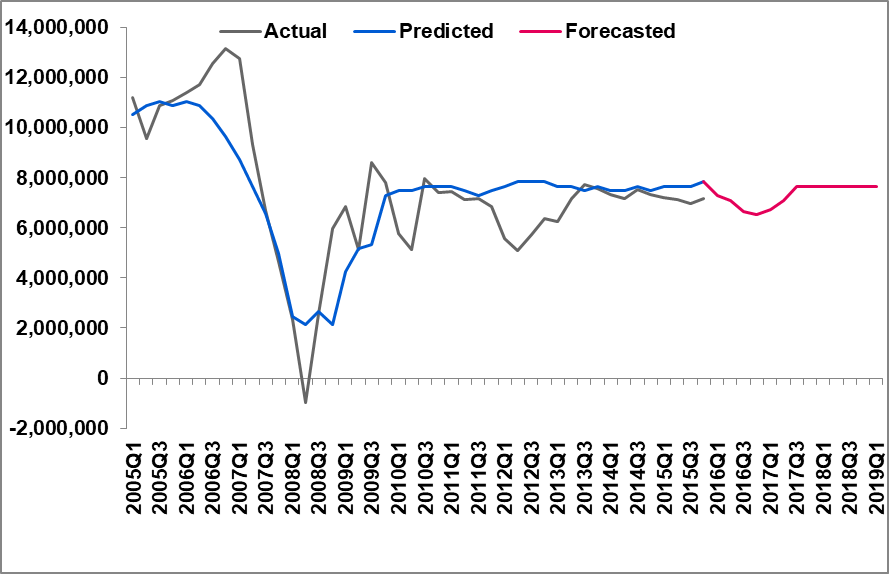
4.5 Projection
The projection is done for 13 Quarters
The dip in 2008-2009 is captured well by the model
The severely adverse projection is done for forecasted period